A) Good atmospheric seeing conditions
On average, seeing conditions in Antarctica are 3-4x better than a comparable mid-latitude ground site [Gillingham, 1993]. The boundary layer varies between 10-40 m (average: 14 m), resulting in 2-3x better spatial resolution and better point sensitivity than a comparable mid-latitude observatory. Antarctic viewing compares favorably even to observatories at high altitude; Mount Haleakalā on Maui, Hawaii (10,023 ft altitude) has median seeing of 0.7 arc-seconds at night. The optical seeing at the South Pole has been measured at 0.46 arc-seconds 7-17 m above the surface, and 0.64 arc-seconds on the surface [Marks et al., 1996]. In other words, viewing from the South Pole is on par with Haleakalā. Antarctic viewing conditions also have low scattered light, high atmospheric transparency, low water vapor, and high sky stability, all resulting in good photometric sensitivity.
B) Long-duration observations with breaks that are essentially random
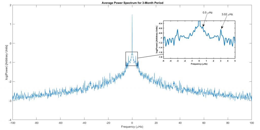
Observations from low-latitude sites are interrupted by the diurnal cycle and associated bad weather. This leads to a time series that is the product of a square-wave-like “on/off” function (also called the “window function”) and the essentially sinusoidal oscillations of the target. The gap structure in the window function due to the diurnal cycle is particularly insidious to any periodogram-based analysis, as it is also periodic. This leads to a spectrum of the observations where each true oscillation line from the target is surrounded by a forest of side-lobes. This side-lobe structure can severely complicate the identification and measurement of the spectral lines from the target. In addition, the lower the fill-factor of the window function the higher the background noise level in the spectrum. Observing from the South Pole has the major advantage that the only interruptions in the observations are from bad weather, and these interruptions are essentially random, which does not lead to any significant side-band structure in the spectrum (see Figure 1).
Moreover, although the average length of time for an uninterrupted observing run is only around 12 hours (Fig. 2), it is possible to obtain observing runs of up to 190 hours without any interruption (Fig. 3).
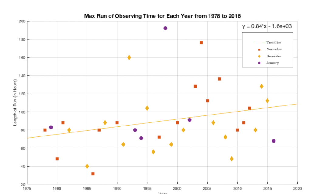
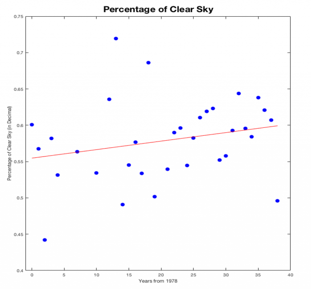
Lastly, the fill factor for observations from the South Pole is significantly higher than can be obtained from a single low-latitude site: with a 37-year average of around 0.58 (see Fig. 3), it is approximately 3x higher than that typically achieved at a low-latitude site.